In this post, we will look at a simple probability model for winning a tennis game. This model is far too simple to be accurate in predicting real tennis matches, but it will be the starting point for building more useful models. It is also a good introduction to some of the more advanced counting techniques used to analyze probability.

Tennis is one of my favorite sports, both to play and to watch. Historically, tennis has lagged behind the major team sports in terms of analytics. This has been changing over the past few years as more analytics professionals focus on the sport. Notably, a research paper on tennis took the prize for best paper at the 2016 MIT Sloan Sports Analytics Conference.

Scoring in Tennis

Compared to other sports, tennis scoring is unusual. In most sports, teams get points, and the team with the most points wins. Simple enough.

In tennis, on the other hand, the player (or players, in the case of doubles) who wins the majority of the sets wins the match (best-of-3 or best-of-5). Because of this, the only points that literally matter in tennis are set points. You could lose the majority of the total points played and in theory still win a tennis match. You just have to win the majority of the set points.

Of course, you have to win enough games to get in a position to win a set. And in order to do that, you have to win enough game points.

As you can see, analyzing tennis requires a hierarchical model. You need to start with analyzing points, and from there move up to the level of games. From games, you then need to move up to the set level. Within the set, you need to think about how the set could end. For tiebreaker sets, you need to analyze tiebreakers, while for advantage sets, you need to think about the fact that the set could last a very, very long time. After dealing with the set analysis, you can start talking about match win probabilities.

Let’s start at the beginning and analyze a single tennis game.

A Simple Model for a Tennis Game

We are going to start with a very simple framework. The simplest possible framework, in fact.

We are going to assume that the server’s probability of winning the next point is some constant. We are going to ignore first serves and second serves for now. We’ll also ignore for the time being the playing surface, and to what side of the court the server is serving. These are all things that matter a lot in real tennis.

We are also going to ignore things like player matchup, fatigue and psychology.

To use realistic numbers, according to this source, Roger Federer has won 69% of his service points on all surfaces over the course of his career. Let’s use this statistic to predict how often the GOAT wins a service game.

Markov Chain Model

We talked about Markov chains in our previous post on the board game Risk.

In that example, we were able to use the fact that the dice probabilities for a given attack don’t depend on what happened previously in the battle. It doesn’t matter whether the attack started 10-on-6 or 50-on-39. If the attacker is down to 3 armies and the defender is down to 2 armies, the dice roll probabilities are the same for either scenario.

If we assume Federer’s chance of winning a service point in a game is always 69%, we can use the same Markov chain framework to analyze that game. At the end of this post, we’ll look critically at this framework, and think about how to extend it to handle more realistic situations.

For now, let’s go with the Markov chain framework and assume Federer’s service point win probability $p = 0.69$ . Starting from a score of 0-0, this means we can look at all possible ways the game can play out. Since pictures are easier to follow than words, here is a depiction of the tennis game Markov chain.

Simple Markov Chain Framework for Tennis Game

This figure presents the Markov chain as a graph. In a graph, the states are depicted as nodes (also called vertices). In the case of tennis, the states are the possible scores in the game. In Risk, the states were how many armies the attacker and defender have left in the battle.

The graph also shows how the states can change using edges. In the case of tennis, the edges are points played. There are two edges coming out of each node; one for the server winning the point, and the other for the returner winning the point. These edges have arrows because they are directed. The score can only change in the directions shown by the arrows. Notice that there are two edges which have double-sided arrows: deuce to ad in, and deuce to ad out. This is because tennis games have to be won by a margin of 2 points after deuce. So, play can alternate between deuce and ads as many times as necessary. In theory, a tennis game could last an infinite amount of time!

The only nodes which don’t have edges coming out of them are “hold” and “break”. For these nodes, the game is over. These nodes are called absorbing states because the graph doesn’t lead anywhere else after you reach that state. In Risk, the absorbing states are when one side or the other had no armies left in the battle.

In case you’re curious how I generated the figure above, here’s a link to the Jupyter Notebook which created it.

Independence

If we assume the probability that Federer wins a service point is constant, then we are also implicitly assuming that each service point is independent.

Notice also that the assumption of constant probability per point is the same as modeling each tennis point as a biased coin toss.

As we will see in future posts, in more realistic models, we can have the independence assumption without necessarily assuming the point win probability is the same for every service point. Constant probability automatically implies independence, but independence doesn’t have to mean constant probability.

We will revisit the issue of independence, and how true it is for tennis, at the end of the post.

Winning a Game

The winner of a tennis game is the first player to win 4 points, unless the score gets to deuce. Deuce occurs for the first time when each player wins 3 points. We will need to examine deuce carefully, since a player has to win by 2 points after a deuce, and the game score can return to deuce any number of times.

Think about the number of ways a server can hold serve. The server can hold to love, hold to 15, hold to 30 or hold after at least one deuce.

These outcomes are each mutually exclusive and exhaustive. For the server to hold, one of these outcomes must happen, and only one can possibly happen in a particular tennis game.

Since the outcomes are mutually exclusive and exhaustive, we are allowed to add the probabilities of each of the outcomes happening. So we can write

$\begin{aligned} P(\textrm{Server holds}) & = P(\textrm{Hold to love}) + P(\textrm{Hold to 15}) + P(\textrm{Hold to 30}) \\ & + P(\textrm{Hold after at least one deuce}) \end{aligned}$

Notice that we lumped together all the possible deuces into that one outcome (“at least one deuce”). You’ll see why in a moment.

Counting Outcomes

Let’s go through each of the above outcomes and figure out their respective probabilities. Then, we can add them up to get the overall probability that the server holds.

Hold to Love

The server holds to love if he or she wins all 4 points in a row. Each point is independent, and the server has probability $p$ of winning each point. We can calculate the joint probability of independent events by multiplying the probabilities. In this case, the probabilities are all the same, so we get

$P(\textrm{Hold to love}) = p^4$

Hold to 15

The server holds to 15 if he or she wins 4 points and the returner wins 1 point.

In this situation, however, we aren’t sure exactly which points the server wins, except for the fifth and last point. All we know is that the server won 3 out of the first 4 points. How do we compute probabilities in this situation?

Notice that there are 4 possible variations: either the returner won the first point, the second point, the third point or the fourth point. Each of these are mutually exclusive and exhaustive outcomes. If the server holds to 15, we know that one of these outcomes must have happened, and that only one could have happened.

Let’s look at the probability of the server holding to 15, assuming that the returner won the first point. The probability of this outcome is

$(1-p) \times p \times p \times p \times p = p^4(1-p)$

Now let’s look at the probability of the server holding to 15, assuming the returner won the second point. This probability is

$p \times (1-p) \times p \times p \times p = p^4(1-p)$

It’s the same! Hopefully that’s no too surprising. The points are independent, so the order in which the returner wins 1 point and loses the other 3 points doesn’t matter. Therefore, the probability of each of the 4 outcomes in which the server holds to 15 is $p^4(1-p)$ .

Since there are 4 mutually exclusive and exhaustive outcomes, we can add them up. Each of these probabilities is the same, so adding them up is the same as multiplying by 4. So, the overall probability of the server holding to 15 is

$P(\textrm{Hold to 15}) = 4p^4(1-p)$

Hold to 30

The same logic applies to the situation where the server holds to 30. There are 6 points played, of which the returner wins 2 of the first 5, the server wins 3 of the first 5, and the server wins the sixth.

The only challenge in this situation compared to the prior examples is the number of outcomes to count goes up a lot. Holding to love only had one outcome to check, while holding to 15 had 4 outcomes to check. Is there a faster way to count the possible outcomes in general?

This question was answered a long time ago. The answer is given by the binomial coefficients. You may have learned about the binomial coefficients first in the context of Pascal’s triangle.

The binomial coefficients show up in a lot of different places in mathematics. In our particular case, we want to know the number of ways the returner can win 2 points out of 5, where the order doesn’t matter. This is given by the binomial coefficient

${5 \choose 2} = 10$

You can get the answer from Pascal’s triangle. Remember that the entries in Pascal’s triangle start from zero. So ${5 \choose 2}$ is in the sixth row, third from the left. The value is 10.

Notice that we get the same answer if we phrase the question in terms of the server. We want to know how many ways the server can win 3 points out of 5, where the order of the points doesn’t matter. This is the binomial coefficient ${5 \choose 3}$ . The answer is also 10. It’s good that both questions have the same answer, because they are two ways of asking the same question.

Now that we know there are 10 possible ways in which the server can hold to 30, it’s easy to figure out the probability of the server holding to 30. Each possible sequence of points has 4 points won by the server, and 2 points won by the returner. Therefore,

$P(\textrm{Hold to 30}) = 10p^4(1-p)^2$

Binomial Coefficients

Before we look at deuce, let’s see what the above 3 cases have in common.

The general formula for the binomial coefficient is

${n \choose k} = \frac {n!} {k!(n-k)!}$

In the above formula, the symbol $!$ denotes the factorial function. The symbol ${n \choose k}$ is usually read “n choose k”, which is a handy reminder of what it means.

Let’s look at this formula for the case of ${5 \choose 2}$ , which we already understand.

$\begin{aligned} 5! & = 5 \times 4 \times 3 \times 2 \times 1 = 120 \\ 2! & = 2 \times 1 = 2 \\ (5-2)! & = 3! = 3 \times 2 \times 1 = 6 \\ {5 \choose 2} & = \frac {120} {2 \times 6} = 10 \end{aligned}$

It’s not a coincidence that ${4 \choose 0} = 1$ and ${4 \choose 1} = 4$ . The coefficients in the probabilities for $P(\textrm{Hold to love})$ and $P(\textrm{Hold to 15})$ are also binomial coefficients.

One last point on the binomial coefficients. If you look at the graph earlier in this post, you can imagine following a path through the graph as each point is played. For each point, you multiply by the probability of going along that edge to the next node. To figure out the probability of holding at 30, you would need to find the number of ways to end up at “hold”, passing through at least one node where the returner has a score of 30, and never passing through deuce or any node where the returner score is 40.

The graph shape (for the points not going through deuce) should remind you a lot of Pascal’s triangle. It’s not a coincidence that the number of paths follows the same pattern.

OK, now we have to handle deuce.

Getting to Deuce

First, let’s figure out the probability of getting at least one deuce. To answer this question, we can use the same counting framework as the previous examples. It’s only after we get to deuce that the situation gets complicated.

To get to the first deuce, we must have played 6 points. The server and returner must each have won 3 points. The binomial coefficient we need is ${6 \choose 3} = 20$ , which you can also obtain by looking at Pascal’s triangle.

Therefore, the probability of getting to deuce in the first place is

$P(\textrm{Get to deuce}) = {6 \choose 3}p^3(1-p)^3 = 20p^3(1-p)^3$

Holding from Deuce

Now that we know the probability of getting to deuce in the first place, we need to think about what can happen next.

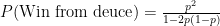
If the server wins 2 points in a row after deuce, the server holds. The probability of the server winning 2 points in a row is $p^2$ .

If the server wins a point and loses a point after deuce, we are back at deuce. There are 2 ways this could happen. The score could go ad in then back to deuce, or the score could go ad out then back to deuce. For each of these two paths, the probability is $p(1-p$ . Therefore, the probability of returning to deuce is $2p(1-p)$ .

Therefore, the probability of winning from deuce is

$P(\textrm{Win from deuce}) = p^2 + 2p(1-p) P(\textrm{Win from deuce})$

Wait, what? The probability $P(\textrm{Win from deuce})$ shows up on both sides of the equation?

Yes, because of the Markov property in our simple model. The probability of winning from deuce, after we play two more points and end up back at deuce, is still the probability of winning from deuce. This sounds like some sort of infinite loop, but the algebra works just fine. (Here is an analysis of deuce that uses an infinite series to get the same answer, but you don’t actually need to use an infinite series.)

Solving,

$P(\textrm{Win from deuce}) = \frac {p^2} {1 - 2p(1-p)}$

Holding via Deuce

Now we can finally solve the probability of holding after at least one deuce. Because all of the points are independent, the probability of holding via deuce is equal to the probability of getting to deuce, times the probability of holding after we get to deuce. As an equation,

$\begin{aligned} P(\textrm{Hold via deuce}) & = P(\textrm{Win from deuce}) \times P(\textrm{Get to deuce}) \\ & = \frac {p^2} {1 - 2p(1-p)} \times 20p^3(1-p)^3 \\ & = \frac {20p^5(1-p)^3} {1 - 2p(1-p)} \end{aligned}$

Putting It All Together

Once we’ve figured out the probabilities of each possible way in which the server can hold, we just need to add them up to get the overall probability of holding serve.

Let’s put this into a simple Python program and plot some results to see how it looks.

A Jupyter Notebook with the code may be found here.

import numpy as np

import matplotlib.pyplot as plt
%matplotlib inline
import seaborn as sns
sns.set()
sns.set_context('notebook')
plt.style.use('ggplot')

def prob_hold_to_love(p):
    """Probability server holds at love."""
    return p**4

def prob_hold_to_15(p):
    """Probability server holds to 15."""
    q = 1-p
    return 4*(p**4)*q

def prob_hold_to_30(p):
    """Probability server holds to 30."""
    q = 1-p
    return 10*(p**4)*(q**2)

def prob_get_to_deuce(p):
    """Probability game gets to deuce at least once."""
    q = 1-p
    return 20*(p**3)*(q**3)

def prob_hold_via_deuce(p):
    """Probability server holds from deuce."""
    q = 1-p
    d = (p**2) / (1 - 2*p*q)
    return d*prob_get_to_deuce(p)

def prob_hold(p):
    """Probability server holds."""
    return (
        prob_hold_to_love(p) +
        prob_hold_to_15(p) + 
        prob_hold_to_30(p) + 
        prob_hold_via_deuce(p)
    )

Let’s generate a plot of the probability that the server holds, as a function of the service point win probability.

PROBS = 25

point_probs = [p for p in np.arange(0, 1+1/PROBS, 1/PROBS)]

hold_probs = [float(prob_hold(p)) for p in point_probs]

fig, ax = plt.subplots(figsize=(10,5))
ax.plot(point_probs, hold_probs, label='server hold probability')
ax.plot(point_probs, point_probs, label='service point win probability')
ax.hlines(0.5, 0, 1, linestyles='dashed', linewidth=0.5, color='k')
TICKS = 10
ax.set_xticks(np.arange(0, 1+1/TICKS, 1/TICKS))
ax.set_yticks(np.arange(0, 1+1/TICKS, 1/TICKS))
ax.set_xlabel('service point win probabilty')
ax.set_ylabel('server hold probability')
ax.set_title(f'Probability server holds vs. service point win probability')
ax.legend(loc='lower right')
plt.show()

Hold Probability versus Service Point Probability

The red line is the probability that the server holds. The blue line is the service point win probability. You see that the game win probability (in red) is much higher than the point win probability if the point win probability is only slightly above 50%.

Let’s check the the simple model using Roger Federer’s career service point win percentage.

p = 0.694
prob_hold(p)

0.8884338858106955

From the same source, Federer’s career service game win percentage is 89%. That’s pretty close to the value predicted by the simple model!

Closing Thoughts

It’s encouraging that this very simple model was close to Federer’s actual career service win percentage. However, we still have a lot of work yet to do before we have a realistic tennis prediction model. We should consider more realistic game win probability models, for instance based upon first and second serve percentages, playing surface and matchup. We also need to build models for tiebreaker, set and match win probabilities.

A big potential criticism of this modelling approach is the assumption that points are independent.

There is some empirical evidence that tennis points are not independent (for example, see here). In future posts we will look at some match data and see if we can determine for ourselves how good an approximation independence is.

Think about what the independence assumption means. It means that if the current game score is 40-30, how the score got to that point is irrelevant. Perhaps the server was previously up 40-0, and then lost 2 points in a row. Or maybe the returner was leading 0-30, and then the server won 3 points in a row. From a psychological perspective, those situations might feel very different to the players. We are also ignoring how important the game is in the context of the set and overall match. If the server blew 2 match points, perhaps the psychology favors the returner to get to deuce and save the match.

These psychological factors, as well as fatigue, are challenging to incorporate in a probability model. They are also a key part about what makes tennis, or sports generally, interesting in the first place. Athletes are not robots or biased coin flippers.

Probability of Winning a Tennis Game

Scoring in Tennis

A Simple Model for a Tennis Game

Markov Chain Model

Independence

Winning a Game

Counting Outcomes

Hold to Love

Hold to 15

Hold to 30

Binomial Coefficients

Getting to Deuce

Holding from Deuce

Holding via Deuce

Putting It All Together

Closing Thoughts

Related

Scoring in Tennis

A Simple Model for a Tennis Game

Markov Chain Model

Independence

Winning a Game

Counting Outcomes

Hold to Love

Hold to 15

Hold to 30

Binomial Coefficients

Getting to Deuce

Holding from Deuce

Holding via Deuce

Putting It All Together

Closing Thoughts

Share this:

Related